Chromatography
Evaporation is an endothermic process undergone by all liquids. This physical state change occurs when the surface molecules gain sufficient kinetic energy to overcome the enthalpy of vaporization. This change is entropically favourable, allowing evaporation to occur below the boiling point of the liquid. In a laboratory environment, evaporation is used to separate, concentrate and purify compounds [1]. Techniques such as distillation and rotary evaporation [2] rely solely upon the evaporation of solvents and their respective properties.
Solvent evaporation is used extensively in sample preparation for chromatography. Solid Phase Extraction (SPE) is a common sample preparation technique [3] where the final eluent is often evaporated [4]. This evaporation step has several benefits for analysis - samples can be reconstituted in a lower volume of solvent which will increase the sensitivity of the method, solvent composition can be modified to improve peak shapes on chromatographic methods and volatile interferences may be evaporated off improving the cleanliness of a sample. These advantages lead to a cleaner, more concentrated sample with less interfering compounds, providing better sensitivity and selectivity.
The requirements for evaporation are broad and some traditional techniques and instruments are not flexible enough to meet the demands. Evaporation in a lab environment has several requirements - being able to work with different numbers of well plates (24, 48, 96, 384 wells), dealing with compounds which are sensitive to heat or atmospheric conditions, as well as a need for sample cleanliness.
This application note uses the Ultravap® Mistral blowdown evaporator (Porvair Sciences product code: 500149) which directs heated gas, typically nitrogen, through a needle head down onto the sample surface to provide gentle evaporation of the solvent. This results in lower thermal degradation of samples since only the surface is heated, with the greater proportion of the sample remaining at ambient temperature. The evaporator consists of several controllable parameters such as gas temperature, gas flow rate and needle position; each of which can be adjusted over time to fit the desired evaporation application.
The Ultravap® Mistral uses heated gas to displace the solvent surface, providing a large surface area for evaporation. Knudsen-Langmuir’s equations [5] show surface area is directly proportional to the rate of evaporation, therefore providing maximum surface area is key for efficient evaporation (equation 1). The needle height of the Ultravap® Mistral can be modified to keep a set distance away from the surface as the solvent evaporates. By tracking the height of the liquid surface during evaporation, maximum displacement can be achieved throughout the entire evaporation run.
Blowdown evaporation provides sufficient kinetic energy directly to the upper surface molecules, allowing them to overcome the enthalpy of vaporization. Consequently, this allows evaporation to occur significantly below the boiling point of the bulk solvent. Therefore, the gas temperature can be set considerably lower than the boiling point, unlike bulk evaporation techniques which provide heat to the entire volume of solvent being evaporated. The rate of evaporation is strongly dependent on the vapour pressure, enthalpy of vaporization and viscosity of the solvent rather than the boiling point. An example of this is hexane which has a relatively high boiling point (69°C) [6], but readily evaporates at room temperature due to the very small enthalpy of vaporization (31.5 kJ/mol @ 25°C) [7] and high vapour pressure (20.1 kPa @ 25°C) [8].
Predicting the effect that gas temperature and gas flow have on the evaporation rate can be challenging. This study was conducted to assess the effect of different conditions on the evaporation rate of a range of solvents. The rate of evaporation was quantitatively assessed and compared through testing a range of temperatures (30, 60 and 80°C), gas flow rates (55 and 75 L/min) to evaporate a range of solvents. Thus, providing insight into efficient and effective evaporation methods with exact needle heights and optimal conditions for fast solvent evaporation.
To determine the rate of solvent evaporation, a non-intrusive method was required subsequently a gravimetric approach was selected. Firstly, the mass of an empty 96 well square 2 mL polypropylene (PP) deep well collection plate (Porvair Sciences product code: 219009) and silicone cap mat (Porvair Sciences product code: 997075SW-96) was measured to 4 decimal places. The cap mat was used to eliminate any unwanted evaporation during the weighing process providing a more accurate measurement.
The Ultravap® Mistral was pre-heated to the desired temperature prior to commencing each experiment, which minimised any temperature differences between tests. 1 mL of solvent was added to the collection plate. The mass of the plate, seal and solvent was determined before placing the plate in the Ultravap® Mistral. The initial needle position was set to be approximately 10 mm above the solvent surface, with a value between 27 mm – 28.5 mm depending on the expansion properties of the solvent. The initial temperature of the solvent, at T = 0 min, was also assumed to be ambient (23°C). A fixed height evaporation method was created for the Ultravap® Mistral in which the needle height would be constant throughout the evaporation run.
After 2-15 minutes, slower evaporating solvents had a longer elapsed time between measurements, the instrument would be stopped, the plate sealed and the mass of the remaining solvent determined. After which, the plate would be placed back into the evaporator and the needle height modified, if necessary, to keep the distance around 10 mm from the surface.
This process was repeated until all the solvent had evaporated. This procedure was repeated using different gas flow rates, temperatures and solvents.
Once all experiments were completed, the plate mass values at each time point were converted to an average volume of solvent per well using equation 2. When plotted against time, the gradient gave an overall average rate of evaporation.
Due to the shape of the collection plate wells, this evaporation rate was subsequently broken down into a top “cuboid” section (section 1) and a lower “cone” section (section 2) (Figure 1).
Figure 1: A schematic of the collection plate well including dimensions used to calculate solvent height and subsequently needle heights. Yellow = Section 1 & Green = Section 2
Solvent volume was converted to height of solvent within the collection plate. This allowed the vertical height of the solvent surface to be monitored over-time. The total internal volume of the 2 mL PP deep well collection plate is 2,300 mm3, with section 1 equalling 2,150 mm3 and section 2 equalling 150 mm3. For volumes greater than 150 µL, the vertical height was found using equation 3.
A different method was required for calculating the height of the solvent surface for volumes below 150 µL, due to the inverted cone shape of the wells. A standard cone volume calculation was not suitable for the calculation as the diameter changes with reducing volume. Due to the symmetrical shape of the cone, the ratio of the height to radius will remain constant, hence a vertical height was calculated using equation 4.
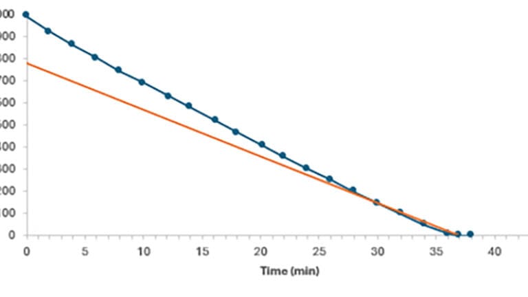
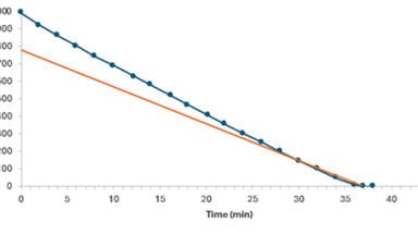
The total evaporation time was determined for each solvent from the x-intercept on each evaporation rate plot, calculated by extrapolation. Figure 2 is an example evaporation rate plot for 100% methanol at 80°C and 55 L/min.
The predicted evaporation time for each water-organic solvent mixture was calculated using the gradient and y-intercept from the evaporation rate plots and the respective volumes of the mixtures and inserted into equation 5.
The following approximations and assumptions were made to allow interpretation of the data:
- The solvent composition was constant throughout the experiment with no change in density
- There was no evaporation during the weighing process
- The cumulative evaporation time, including pauses for weighing, was comparable to uninterrupted evaporation
- The mass of the plate and seal was constant throughout the experiment
- Each well evaporated at the same rate
- The initial temperature of the solvent was the same for all experiments
Solvents used in the study are detailed in Table 1 below:
A higher temperature yielded a faster overall rate of evaporation than a lower temperature for every solvent tested at both gas flow rates (55 L/min and 75 L/min). An example of this trend, using 55 L/min gas flow rate data, is shown in figure 3 and table 2. Figure 3: Chart showing the evaporation rate in µL/min at three gas temperatures (30, 60 and 80°C) at a gas flow rate of 55 L/min
When comparing the percentage increase in evaporation rates between the 30°C to 60°C and 60°C to 80°C ranges at a gas flow rate of 55 L/min (figure 4 and table 3), the increase from 30°C to 60°C was generally much larger. This remains true even when accounting for the increase per °C. This trend is likely because the larger increase from 30°C to 60°C introduces a larger relative amount of kinetic energy to the molecules. In contrast, at 60°C to 80°C, the solvent molecules already have a significant amount of kinetic energy, so the increase in rate is not as high. This same trend was seen at a gas flow rate of 75 L/min.
This trend did not apply to methanol, this is likely due to the large increase in vapour pressure at 75°C, compared to 25°C (table 1). This is much larger than any of the other solvents tested and would explain the higher increase in evaporation rate at the higher temperature compared to the other solvents. This observation was also seen at 75 L/min.
An increase in gas flow rate yielded a faster overall rate of evaporation than a lower flow rate at every temperature (30, 60 and 80°C). An example of the data at 60°C is shown in figure 5 and table 4.
For mixtures containing 75%, 50%, and 25% methanol, the data at all temperatures indicated that increasing the gas flow rate from 55 L/min to 75 L/min had less impact on the evaporation rate compared to pure methanol. This is likely linked to the viscosity of the solution - the higher the viscosity, the less impact the flow rate had. A higher viscosity solution requires a higher force to displace the surface of the liquid. Therefore, increasing the flow rate would result in less displacement and surface area for evaporation, lowering the rate of evaporation.
An interesting finding of this study was how differently water interacts with methanol compared with acetonitrile during evaporation. Figure 6 shows that for acetonitrile, two linear sections of evaporation are observed – between 0 and ~16 minutes and from ~16 minutes until ~78 minutes. This suggested acetonitrile evaporated off first, followed by water which evaporates at a slower rate reducing the overall evaporation rate. However, for methanol-water mixtures a curve can be seen. The reason for this difference could be the water hydrogen bonding to the methanol, forming clusters [29] and larger hydrogen bonded species. This would increase the energy required to break the hydrogen bonds to allow solvent to evaporate. Whereas acetonitrile-water solutions form stronger [30], but fewer hydrogen bonds, resulting in weaker cluster formation.
It was hypothesised that evaporation times for mixtures of solvents could be predicted through extrapolation of the pure solvent evaporation rates and calculated using equation 5.
In the case of an acetonitrile-water solution, this gives a reasonable estimate of the evaporation time (figure 7A) where there is only a 6.3% difference in time between the predicted and experimental values. However, with a methanol-water mixture, this was not the case with it taking longer for the mixtures to evaporate compared to the predicted evaporation time (figure 7B). A percentage difference of 28.0% was observed between theoretical and experimental values. This shows that a prediction is not simple due to the different interactions between the two solvents which have been outlined above - the increase in viscosity combined with hydrogen bonding which results in a slower than expected evaporation time. Further to this, acetonitrile had the same difference between predicted and experimental values at all concentrations. However, methanol differed more from the predicted value the higher the percentage of methanol in the solution (table 5).
Evaporation rates of common chromatography solvents using the Ultravap® Mistral blowdown evaporator were evaluated at a range of temperatures and gas flow rates. The results showed that temperature significantly increases the evaporation rate, while higher gas flow rates also contribute, albeit to a lesser extent. Additionally, the study highlighted differences in evaporation dynamics between solvent mixtures, acetonitrile-water and methanol-water, likely due to the interaction between methanol and water. The data collected can be used to optimise evaporation methods, such as needle height settings, temperature and flow rate conditions on the Ultravap® Mistral, and to improve the prediction of solvent evaporation times for different solvent and solvent-water mixtures.
[1] D. J. Chantel C. Tester, “Chapter Twelve - Precipitation in Liposomes as a Model for Intracellular Biomineralization,” Methods in Enzymology, vol. 532, pp. 257-276, 2013.
[2] E. P. H.L. Lord, “Sample Preparation Automation for GC Injection,” Comprehensive Sampling and Sample Preparation, pp. 597-612, 2012.
[3] J. Edwards, “Is Poor Sample Prep Impacting Your Bioanalytical Methods?,” [Online]. Available: https://www.microplates.com/resources/. [Accessed 15 October 2024].
[4] J. Edwards, “Microlute® CSi: Evaluation of a Novel,” [Online]. Available: https://www.microplates.com/resources/. [Accessed 15 October 2024].
[5] K. W. Kolasinski, Surface Science: Foundations of Catalysis and Nanoscience, 3rd ed., 2012, p. 203.
[6] W. Haynes, CRC Handbook of Chemistry and Physics., 91st ed., C. P. Inc., Ed., 2010-2011, pp. 3-282.
[7] V. Majer and V. Svoboda, Enthalpies of Vaporization of Organic Compounds: A Critical Review and Data Compilation, Oxford: Blackwell Scientific Publications, 1985, p. 300.
[8] C. Williamham, W. Taylor, J. Pignocco and F. Rossini, “apor Pressures and Boiling Points of Some Paraffin, Alkylcyclopentane, Alkylcyclohexane, and Alkylbenzene Hydrocarbons,” vol. 3, no. 35, pp. 219-244, 1945.
[9] Anton-Paar, “Viscosity of Acetonitrile,” [Online]. Available: https://wiki.anton-paar.com/kr-en/acetonitrile/. [Accessed 15 October 2024].
[10] Anton-Paar, “Viscosity of Methanol,” [Online]. Available: https://wiki.anton-paar.com/kr-en/methanol/. [Accessed 15 October 2024].
[11] Anton-Paar, “Viscosity of Water,” 2008. [Online]. Available: https://wiki.anton-paar.com/kr-en/water/. [Accessed 15 October 2024].
[12] O. Bridgeman and E. Aldrich, “Vapor Pressure Tables for Water,” J. Heat Transfer, vol. 86, no. 2, pp. 279-286, 1964.
[13] CRC, Handbook of Chemistry and Physics, 44th ed., CRC Press, 1962.
[14] C. E. R. I. Center, “Pure Component Properties,” 2007. [Online]. Available: https://en.wikipedia.org/wiki/Acetonitrile_(data_page). [Accessed 15 October 2024].
[15] C. S. R. T. D Ambrose, “Thermodynamic properties of organic oxygen compounds XXXVII. Vapour pressures of methanol, ethanol, pentan-1-ol, and octan-1-ol from the normal boiling temperature to the critical temperature,” The Journal of Chemical Thermodynamics, vol. 7, no. 2, pp. 185-190, 1975.
[16] J. Dojcansky and J. Heinrich, “Saturated Vapour Pressure of Acetonitrile,” Chem. Zvesti, vol. 2, no. 28, pp. 157-159, 1974.
[17] X. Ge and X. Wang, “Estimation of Freezing Point Depression, Boiling Point Elevation, and Vaporization Enthalpies of Electrolyte Solutions,” Industrial & Engineering Chemistry Research, vol. 48, no. 10, p. 5123, 2009.
[18] T. J. K. J. W. J. J. Will Thompson, “Viscosity measurements of methanol–water and acetonitrile–water mixtures at pressures up to 3500bar using a novel capillary time-of-flight viscometer,” Journal of Chromatography A, vol. 1134, no. 1-2, pp. 201-209, 2006.
[19] The Engineering ToolBox [online], “https://www.engineeringtoolbox.com/surface-tension-d_962.html,” 2005. [Online]. Available: https://www.engineeringtoolbox.com/surface-tension-d_962.html. [Accessed 15 October 2024].
[20] J. Urban, “Mobile Phase Viscosity,” 2010. [Online]. Available: http://www.chromatographer.com/mobile-phase-viscosity/. [Accessed 15 10 2024].
[21] “Vapor Pressures of Acetonitrile Determined by Comparative Ebulliometry,” Journal of Chemical & Engineering Data, vol. 49, no. 3, pp. 486-491, 2004.
[22] H. Hu, C. R. Weinberger and Y. Sun, “Effect of Nanostructures on the Meniscus Shape and Disjoining Pressure of Ultrathin Liquid Film,” Nano Letters, vol. 14, no. 12, pp. 7131-7137, 2014.
[23] NIST, “NIST Chemistry WebBook, Acetonitrile,” [Online]. Available: https://webbook.nist.gov/cgi/cbook.cgi?ID=C75058&Mask=4. [Accessed 15 October 2024].
[24] NIST, “NIST Chemistry WebBook, Methyl Alcohol,” [Online]. Available: https://webbook.nist.gov/cgi/cbook.cgi?ID=C67561&Units=SI&Mask=4#Thermo-Phase. [Accessed 15 October 2024].
[25] NIST, “NIST Chemistry WebBook, Water,” [Online]. Available: https://webbook.nist.gov/cgi/cbook.cgi?ID=C7732185&Mask=4. [Accessed 15 October 2024].
[26] A. P. R. S. Jagannath Pal, “Thermodynamic properties of forming methanol-water and ethanol-water clusters at various temperatures and pressures and implications for atmospheric chemistry: A DFT study,” Chemosphere, vol. 272, 2021.
[27] N. G. S. C. M. V. David, Advances in Chromatography, vol. 54, boca raton: CRC Press, 2018.
[28] V. Gonzalo, A. Estrella and J. M. Navaza, “Surface Tension of Alcohol Water + Water from 20 to 50 .degree.C,” Journal of Chemical & Engineering Data, vol. 40, no. 3, pp. 611-614, 1995.
[29] DataPhysics Instruments GmbH, “Surface tension values of some common test liquids for surface energy analysis,” [Online]. Available: https://www.dataphysics-instruments.com/Downloads/Surface-Tensions-Energies.pdf. [Accessed 15 October 2024].
[30] D. R. Stull, “Vapor Pressure of Pure Substances. Organic and Inorganic Compounds,” Ind. Eng. Chem., vol. 39, no. 4, pp. 517-540, 1947.
ILM 51.6 Sept 2026


 Product directory











.jpg)